How to use data validation in Google Sheets

Data validation in Google Sheets lets you decide what people can type into your cells. You set a rule once, and Sheets warns about or rejects anything that doesn’t fit, like a misspelled department or a date in the wrong format.

It helps most when several people work in the same spreadsheet, because you catch mistakes as they’re typed instead of cleaning them up later. This guide explains what data validation is, how to add a rule, how each criterion works, and how to copy, edit, and remove rules.

What is data validation in Google Sheets?

Data validation in Google Sheets is a set of rules that controls what people can enter in a cell or range. You choose the cells and a criterion, such as a dropdown list, a number range, or a valid date. Sheets then flags or rejects any entry that breaks the rule.

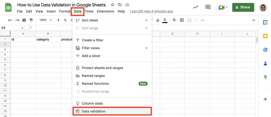
You’ll find it under Data > Data validation, which opens the rules in a sidebar on the right.

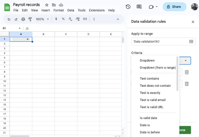
Let’s take a look at each element within the data validation feature:

Apply to range: This is the range of cells your data validation will be applied to.
Criteria: This is the type of data validation you want to apply. The options are the following: Dropdown, Dropdown from a range, Text, Date, Number, Custom formula, and Checkbox. You will see an in-depth explanation in the section on How to do data validation in Google Sheets.
Advanced options: Optional help text for the cell, and whether Sheets shows a warning or rejects the input when the data is invalid.

Data validation in Google Sheets — Criteria list in the Data validation rules sidebar, from Dropdown to Date is before

Why validate your data in Google Sheets?

There are many reasons why you should use data validation in Google Sheets. Here are some of the most important benefits:

Accurate data: By setting up parameters around data input, users will not be able to input the wrong data or formatting without Google Sheets either recognizing this or rejecting the input entirely.
Consistent data: You can make sure each row of data follows the same rules by adding specific data ranges – for example, if dealing with percentages, you can adjust the data range so that no user can input a value over 100.
Save time from editing: Because this feature controls the data for you, there is no need to read through and edit any incorrect data, saving you a lot of time.
Control other users’ inputs: Data validation is particularly helpful if you are sharing your Google Sheets file with others, or receiving data from other sources. You will have full control over what data they can and cannot enter.

Use case

These benefits apply to everyday data management, so data validation can indeed be used in almost any spreadsheet process and use case.

For example, let’s say I am in charge of collecting employee data to monitor monthly salary payments. I can use data validation to control the type of input received, such as the formatting of their date of birth, the department they belong to, or their employee ID.

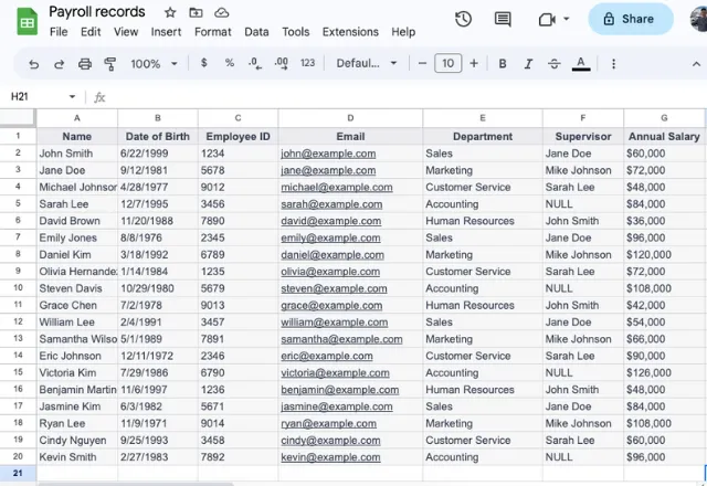
Data validation in Google Sheets — payroll sheet with names, dates of birth, employee IDs, emails, and departments

With data validation, there is no risk of accidental errors from manual input, or employees inputting incorrect data.

As a result, I will have a large file of accurate, employee data that I don’t have to read through and edit, ultimately saving me hours of work.

How to add a data validation rule in Google Sheets

In Google Sheets, you can add and manage your data validation rules by going to Data > Data validation.

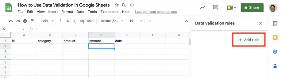
Data validation in Google Sheets — Data menu open with Data validation highlighted

From the side panel, click ‘Add rule’ to start a new rule.

Data validation in Google Sheets — empty Data validation rules sidebar with the Add rule button

Below, you will learn about the options available and how to add a simple rule: the ‘amount’ value must be greater than zero.

Apply to range

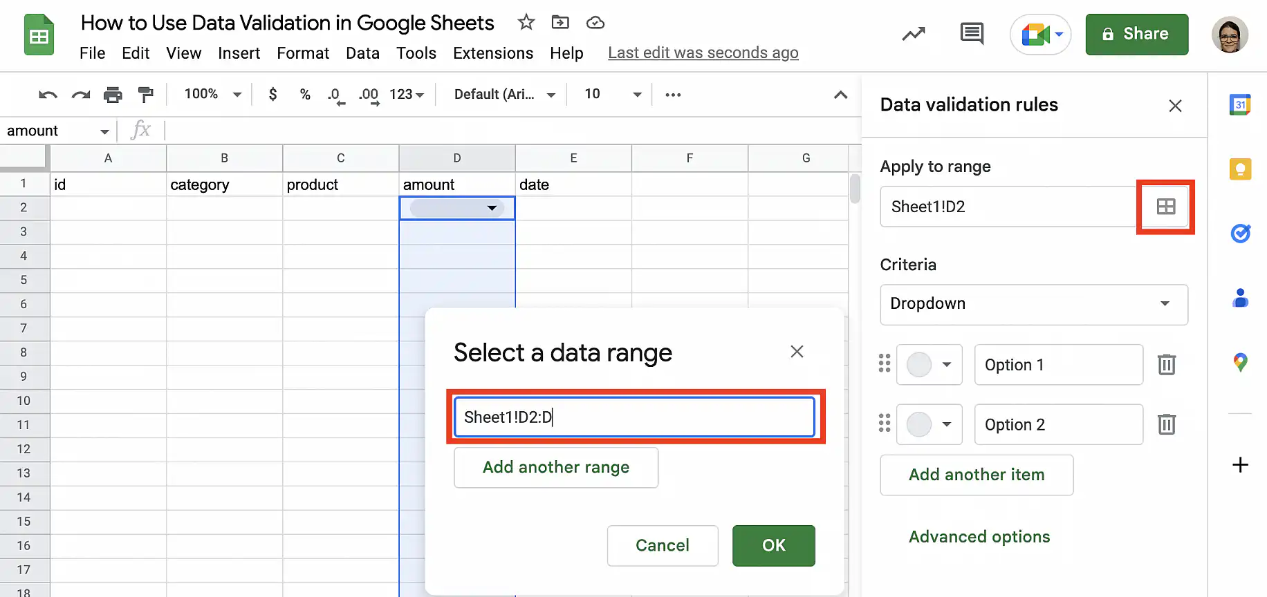
In the ‘Apply to range’ box, select the cell or range of cells to which you want to apply the data validation rule. Alternatively, you can select the cells before adding the rule. Below, I have selected everything but the header in column D. To pick the cells with your mouse, click the grid icon at the end of the box, select them, and click ‘OK’.

Data validation in Google Sheets — Select a data range dialog set to Sheet1!D2:D

Criteria

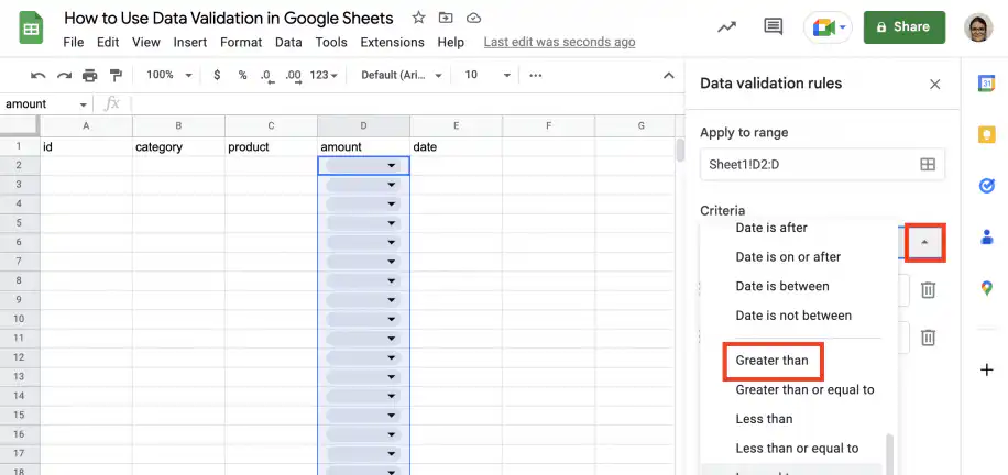
There are multiple options for adding criteria. Click the downward pointing arrow to select from the drop-down menu. In this case, I want the ‘greater than’ option.

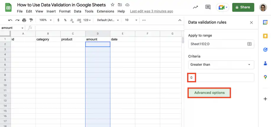
Type zero in the value box, as shown below. Click ‘Done’ to apply or click ‘Advanced options’ to see more options.

Data validation in Google Sheets — Greater than criterion with the value 0 and the Advanced options button

Advanced options: show a warning or reject the input

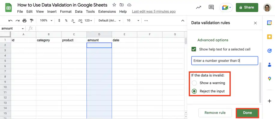
The advanced options allow you to specify what happens when invalid input is entered. First, check the box to ‘Show help text for a selected cell’. You can use the suggested message or type your own.

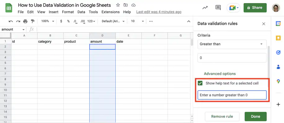
Data validation in Google Sheets — help text Enter a number greater than 0 under Advanced options

Next, you can choose whether to show a warning or reject the input. The help text shows in either case. With ‘Show a warning’, Sheets keeps the entry but marks the cell with a red triangle and an Invalid note. With ‘Reject the input’, Sheets blocks the entry and shows an error message, so the cell keeps its previous value. Click ‘Done’ to apply the validation rule.

Google Sheets data validation reject input option — Reject the input selected under If the data is invalid

How to do data validation in Google Sheets

Let’s use the use case above to go through a step-by-step data validation process.

As mentioned previously, there are several different criteria for data validation in Google Sheets.

Let’s go through each of these to understand exactly what they do and what they may look like inside your own Google Sheets file, using the use case mentioned above.

Dropdown and dropdown from a range

This is the option to create a pull-down menu in the sheet by inputting the choices manually. For colors and dependent lists, see this guide to dropdown lists in Google Sheets.

First, under Criteria, select Dropdown.

Then choose the range of cells where you want to create the dropdown list.

Add the text to the boxes. In this example, I’ll add all the departments.

Dropdown data validation in Google Sheets — Dropdown criterion on E2:E1000 with Sales as the first item

You can also pick a different color for each option. To color a whole row based on the option someone picks, use conditional formatting based on another cell.

Dropdown data validation in Google Sheets — color palette open for a dropdown item

If you prefer, you can select the options from a range of cells instead of typing all the text in the boxes.

In this case, select Dropdown (from a range) in the Criteria section.

After selecting the range where you want to create the dropdown, choose the range of cells containing all the options you need to add to the list.

Dropdown from a range in Google Sheets — Select a data range dialog set to the Departments list in L2:L6

Once I have applied this, you will see my dropdown now contains all the departments. I’ll click Done to create the dropdown list.

Dropdown from a range in Google Sheets — the five departments loaded as items in the sidebar

Now, I don’t need to input the data manually. All I need to do is choose one of the options from the dropdown list.

Data validation in Google Sheets — Department dropdown open in E2 with five options

Text

The Text criterion allows you to control the type of text a user inputs into a cell range. This criterion gives you a lot of options of how to control data, from only accepting an exact text match, to accepting a valid email address or URL.

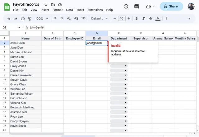
In this example, I can ensure employees input a valid email address in my ‘Email’ column by selecting Text is valid email.

Under Advanced options, you can choose what will happen if I input invalid data. Google Sheets can show a warning or reject the input when the data is invalid.

I’ll choose Show a warning and click Done.

Text data validation in Google Sheets — Text is valid email on D2:D1000 with Show a warning selected

Now if I input invalid data, Google Sheets will show a warning message.

Text data validation in Google Sheets — Invalid warning: Input must be a valid email address

Date

The Date criterion helps you make sure only valid dates are added to the cells and even lets you control date inputs before or after a certain date, or between certain dates.

For example, let’s say in my “Date of Birth” column, I want to make sure that each employee adds their dates correctly. By choosing the Date criterion and the Is valid date option, any invalid dates will be rejected by Google Sheets.

Date data validation in Google Sheets — Is valid date criterion on B2:B1000

Now Google Sheets will only accept a valid date when you input data into the cells where the data validation is applied. If you double-click a cell within this range, a calendar will appear.

Date data validation in Google Sheets — calendar picker open in the Date of Birth column

Number

The Number criterion allows you to define a range of numbers that users can input. You have options to validate numbers above or below a certain value, or between two values.

For example, in my “Employee ID” column, I want to make sure that employees correctly add their 4-digit ID number. I can choose Number is between and add the lowest value as 1000 and the highest as 9999.

This means that users can only input a 4-digit number.

Number data validation in Google Sheets — Is between 1000 and 9999 on the Employee ID column

Checkbox

The Checkbox criterion is perhaps the most straightforward data validation. It allows you to format the cell as a checkbox.

For example, let’s say I want to add a checkbox to my ‘Paid?’ column so that employees can check this when they have received their paycheck. Simply select the Checkbox criterion as shown below.

Checkbox data validation in Google Sheets — Checkbox criterion on I2:I1000, the Paid? column

How to copy data validation rules in Google Sheets

Copying data validation to other cells is simple. First, select the cell or cells with the data validation. Right-click on the cell and select copy or press Ctrl + C (Cmd + C on a Mac).

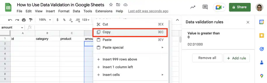
Copy data validation in Google Sheets — right-click menu on D2 with Copy highlighted

Paste to the cell where you want to add the rule. To paste only the rule and keep the target cells’ values and formatting, right-click and choose ‘Paste special’ > ‘Data validation only’.

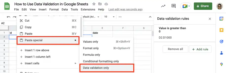
Copy data validation rules in Google Sheets — Paste special menu with Data validation only highlighted

As you can see, the new range has been added to the existing data validation rule.

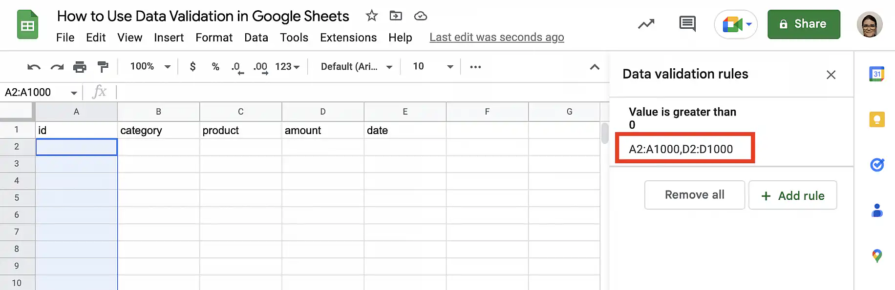
Copy data validation in Google Sheets — rule now applied to A2:A1000 and D2:D1000

You can also copy a rule with the fill handle. Select the cell with the rule and drag the small square in its bottom-right corner over the cells you want to cover. The cell’s value is copied along with the rule, so start from an empty cell if you only want the rule.

To apply a rule to a whole column, open it in the sidebar and change Apply to range to an open-ended range such as Sheet1!D2:D. Leaving out the last row number covers every row below the header, including rows you add later.

Copy and paste also works between sheets in the same file. On the other sheet, Paste special > Data validation only creates a new rule with the same criteria.

How to edit data validation in Google Sheets

You can edit any aspect of your existing rules by going to Data > Data validation. From the side panel, select the rule you want to edit.

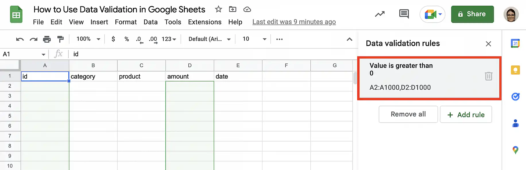
Edit data validation in Google Sheets — Value is greater than 0 rule selected in the sidebar

You will see the same options as when you created the rule. Change the range, the criteria, or the advanced options, then click ‘Done’ to save.

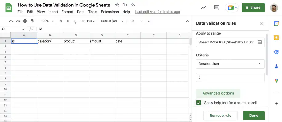
Edit data validation in Google Sheets — rule options with Apply to range, Greater than 0, and help text

How to remove data validation in Google Sheets

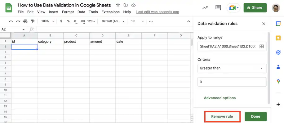
Removing data validation is simple. Go to Data > Data validation and hover over the rule you want to delete in the side panel. Click the trash can icon to delete.

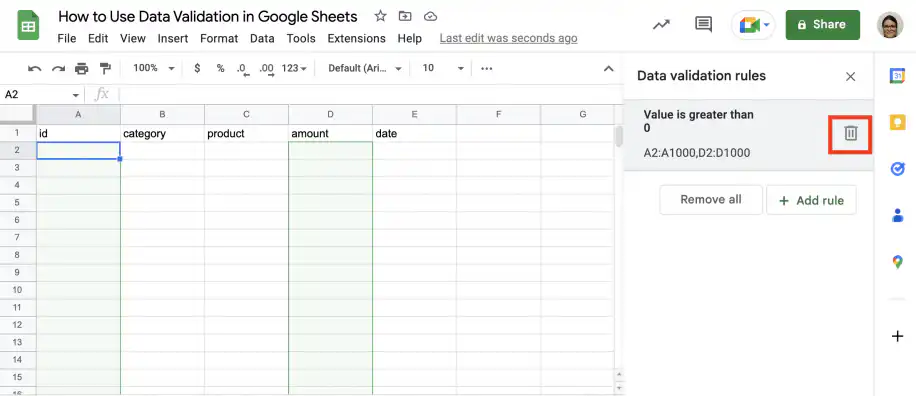
Alternatively, select the rule and click ‘Remove rule’ to delete it. To delete every rule in the list at once, click ‘Remove all’. Either way, the values already in the cells stay where they are.

Remove data validation in Google Sheets — Remove rule button below the open rule

Why is my data validation not working?

If you can’t change the data validation options, check your access first. You need edit access to the file, and the cells can’t sit in a range someone else has protected. Go to Data > Protect sheets and ranges to see what’s locked, or read how to protect cells or pages in Google Sheets. If a specific rule is not applied, check whether the current cell is in the rule’s cell range. Go to Data > Data validation to check. A regular paste can also remove a rule: when you paste a cell without validation over one that has it, the rule is replaced. Use ‘Paste special’ > ‘Values only’ to keep the rule.

Collect validated data with Sheetgo Forms

Data validation protects a spreadsheet that people edit directly. When the data comes from people who shouldn’t open the spreadsheet at all, like field teams or clients, a form is a safer way in.

Sheetgo Forms checks each answer against the rules you set and adds every response to Google Sheets as a new row. You share the form, not the spreadsheet. From there, Sheetgo’s AI-powered workflows carry the data into the reports and files your team uses, so it stays clean and AI-ready from the first entry.

Find out why Sheetgo Forms offer a better alternative to Google Forms.

How to validate data in Google Sheets?

And there you have it! Now you should be able to validate your own data inside Google Sheets using any of the several criteria demonstrated above. You will find that by using data validation, you not only have more control over data when other users input into your sheets, but you also save the time you’d usually spend reviewing and editing your data.

If you would like to learn more about the various features of Google Sheets, why not start with our article on Sorting and filtering data in Google Sheets?

Alternatively, take a look at our related blog posts below!